Understanding the data

C-MLP2LN, Constructive MLP converted to Logical Network

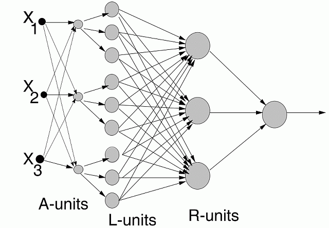
Architecture:

• Aggregation,
• Linguistic variables
• Rule layers;
• one output per class.

Aggregation: used to combine and discover new useful features.
Used only if rules with the given features are not successful.
Constraints: combinations of features of the same type, combinations making sense.

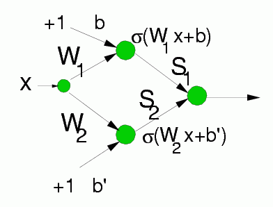
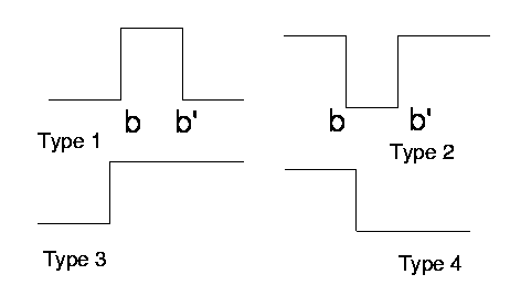
L-units: providing intervals for fuzzy or crisp membership functions
Made from 2 neurons, only biases are adaptive parameters here.

Without L-units decision borders will be arbitrary hyperplanes made by combinations of inputs - sometimes it may be advantageous.
Used only with continuous inputs; if good discretization provided may not be necessary.
Great to optimize linguistic variables together with the rules.

Constraint MLP cost function

First term: standard quadratic error function (or other cost functions)
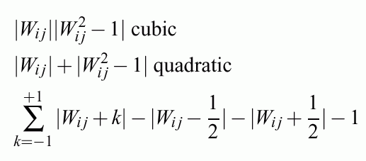
Second regularization term: weight decay & feature selection.
Third regularization term: from complex to simple hypercuboidal classification decision regions for crisp logic (for steep sigmoids).

Different regularizers may be used but there is not much difference in practice.

Different error functions may be used: quadratic, entropy based etc.
Very simple modification of the standard BP required

Increase the slope of sigmoidal functions during learning to get rectangular decision borders.

Another approach: increase a in the regularization term:

This prunes the network leaving large weights, which is equivalent to increasing the slope.

Without logical inputs this allows large but non-equal weights.
What makes the decision borders perpendicular to axis?

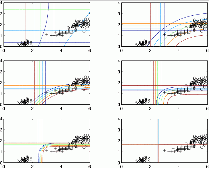
Logical rules from MLP: simplify the network by enforcing weight decay and other constraints.
Strong and weak regularization allows to explore simplicity-accuracy tradeoff.

• Constructive C-MLP2LN algorithm: faster, train one R-unit at a time.
• Add one neuron and train it, freezing the existing skeleton network.
• The network first grows, then shrinks; stop when the number of new vectors per one new neuron becomes too small.

Algorithm:

1. Create one hidden neuron (R-unit neuron).
2. Train the neuron on data for the first class using BP with small l₁=10^-5, l₂=0, and small slope, T=1.
3. If convergence is slow train 2 or more neurons simultaneously.
   1. Train as long as the error decreases; then increase 10 times l₁, increase T+1, train further;
      repeat this step until sharp increase of the error (typical more than 5 times) is noticed when l₁ is increased.
   2. Step back with l₁ and train until convergence.
   3. Remove weights smaller than |W|<0.1.
   4. Take l₂=l₁ and l₁=0, train slowly increasing the slopes and l₂ until all weights reach 0 ±0.05 or ±1±0.05.
   5. Set very large slopes T=1000 and integer weights 0, ±1.
4. Analyze the weights/thresholds to find logical rules covering most common input-output relations.
5. Freeze weights of existing neurons during further training.
6. Add next neuron, train on the remaining data.
   Connect it to the output neuron for its class.
7. Repeat until all data are correctly classified, or too many rules are produced.
8. Repeat the whole procedure for data belonging to other classes.

Many equivalent sets of rules may be found.

Non-gradient optimization methods - closer to global optimum, better rules?
So far poor results but more experiments are needed - use Alopex?

Summary

• Constructive algorithm is fast and requires little experimentation with network construction.
• Sets of rules of different complexity may be created.
• Sets of rules of different rejection rate/reliability are constructed.

Iris step by step

Włodzisław Duch