Most popular benchmark, Fisher 1936.
4 measurements in cm, with accuracy of 0.1 cm.
petals and sepals of 3 kinds of Iris flowers.
50 examples from each class.
Example of Iris data:
| 5.1,3.5,1.4,0.2, Iris-setosa | 6.0,2.2,4.0,1.0, Iris-versicolor | 6.4,2.7,5.3,1.9, Iris-virginica |
| 4.9,3.0,1.4,0.2, Iris-setosa | 6.1,2.9,4.7,1.4, Iris-versicolor | 6.5,3.2,5.1,2.0, Iris-virginica |
| 4.7,3.2,1.3,0.2, Iris-setosa | 5.9,3.0,4.2,1.5, Iris-versicolor | 7.2,3.6,6.1,2.5, Iris-virginica |
| 4.6,3.1,1.5,0.2, Iris-setosa | 5.0,2.0,3.5,1.0, Iris-versicolor | 6.7,2.5,5.8,1.8, Iris-virginica |
| 5.0,3.6,1.4,0.2, Iris-setosa | 5.2,2.7,3.9,1.4, Iris-versicolor | 7.3,2.9,6.3,1.8, Iris-virginica |
| 5.4,3.9,1.7,0.4, Iris-setosa | 6.6,2.9,4.6,1.3, Iris-versicolor | 6.5,3.0,5.5,1.8 Iris-virginica |
| 4.6,3.4,1.4,0.3, Iris-setosa | 4.9,2.4,3.3,1.0, Iris-versicolor | 4.9,2.5,4.5,1.7, Iris-virginica |
| 5.0,3.4,1.5,0.2, Iris-setosa | 6.3,3.3,4.7,1.6, Iris-versicolor | 7.6,3.0,6.6,2.1, Iris-virginica |
| 4.4,2.9,1.4,0.2, Iris-setosa | 6.2,2.2,4.5,1.5, Iris-versicolor | 6.5,3.0,5.8,2.2, Iris-virginica |
| 4.9,3.1,1.5,0.1, Iris-setosa | 5.6,2.5,3.9,1.1, Iris-versicolor | 6.3,2.9,5.6,1.8, Iris-virginica |
Naive: divide into few bins.
Used frequently in fuzzy logic.
Results: usually disastrous!
Example: 3 fuzzy membership functions: 9 fuzzy rules, 26 conditions
5 fuzzy membership funct.: 104 fuzzy rules, 368 conditions
Ref: REFuNN - fuzzy rules extraction, N.K. Kasabov, Fuzzy sets and systems 82 (1996)
Histograms
Display a histogram counting number of vectors in a bin for each class.
Problems: histograms depend on the bin size.
For small number of vectors hard to find good bin size, holes in histograms.
Solution: smooth histogram, treat each vector as a Gaussian of some width and sample K more vectors from this distribution.
Simpler: add a fraction of a vector to adjacent bins.
Example: histograms for Iris
Linguistic variables from smoothed histograms.
SL=x1=Sepal Length; SW=x2=Sepal Width
PL=x3=Petal Length; PW=x4=Petal Width
|
By chance dividing each [min,max] interval in 3 parts gives good results!
Many fuzzy methods do it and Iris is their favorite example!
Result: 12 logical variables instead of 4 continous,
xi => (si, mi, li)
Coding: si=0, 1 or better for neurl networks -1,+1
Conflicts: discretization makes some vectors from different classes identical.
Ex: 3 iris-versicolor vectors, (m,m,l,l), (m,l,m,l) and (m,s,l,m) are identical with some iris-virginica vectors.
Maximum classification accuracy is reduced to 98.0% (3 errors).
2 linguistic variables/feature give 13 conflict vectors.
4 linguistic variables/feature give 16 Iris-versicolor cases = Iris-virginica.
Other methods of linguistic variables determination
Decision trees, clusterization methods, dendrograms.
In the Iris case dendrogram initialization, FSM with Gaussians, gives 95% accuracy, 4 fuzzy rules.
Note: these are initial variables only.
Final values are obtained after rule optimization and should be context dependent i.e. different in each rule, unless for some reason we want the same variables everywhere.
12 input nodes, 3 output nodes, no hidden - single neuron per class is sufficient.
Network trained for 1000 epochs, final weights 0±0.05,
±1±0.05.
| Setosa | (0,0,0 | 0,0,0 | +,0,0 | +,0,0) | Th=1 |
| Versicolor | (0,0,0 | 0,0,0 | 0,+,0 | 0,+,0) | Th=2 |
| Virginica | (0,0,0 | 0,0,0 | 0,0,+ | 0,0,+) | Th=1 |
Rules:
|
Last rule: classifies 53 cases as Virginica, 3 are wrong.
This rule makes 3/50 = 6% errors, 94% correct.
Overall accuracy of the 3 rules is 98%, maximum for this discretization.
Rules should be simplified:
|
Looks good but solution may be brittle, PL=s is in [1,2].
Decision border for Setosa is too close to the data.
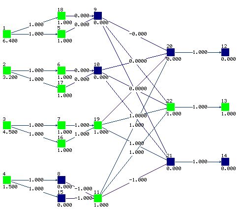
Architecture of the network:
Network structure is more complex since each L-unit provides 2 adaptive parameters
Learning process
| Learning | 0.2 |
| Forcing zeros | 0.00001 |
| Forcing ones | 0 |
| Sigmoid Slope | 2 |
| Learning | 0.2 |
| Forcing zeros | 0.0001 |
| Forcing ones | 0 |
| Sigmoid Slope | 2 |
| Learning | 0.2 |
| Forcing zeros | 0.0005 |
| Forcing ones | 0 |
| Sigmoid Slope | 2 |
| Learning | 0.1 |
| Forcing zeros | 0 |
| Forcing ones | 0.0005 |
| Sigmoid Slope | 2 |
| Learning | 0.1 |
| Forcing zeros | 0 |
| Forcing ones | 0.001 |
| Sigmoid Slope | 2 |
| Learning | 0.01 |
| Forcing zeros | 0 |
| Forcing ones | 0.01 |
| Sigmoid Slope | 4 |
| Learning | 0.001 |
| Forcing zeros | 0 |
| Forcing ones | 0.1 |
| Sigmoid Slope | 4 |
| Learning | 0.0001 |
| Forcing zeros | 0 |
| Forcing ones | 0.1 |
| Sigmoid Slope | 6 |
| Learning | 0 |
| Forcing zeros | 0 |
| Forcing ones | 0 |
| Sigmoid Slope | 1000 |
x1 and x2 have no influence on the output
Biases create windows: x3 Ł2.5 and
x4Ł1.7
Final rules: 5 errors:
IF (x3 Ł2.5 & x4Ł1.7) Iris setosa
IF (x3 >2.5 & x4Ł1.7) Iris versicolor
IF (x3 >2.5 & x4>1.7) Iris virginica
Rules should be simplified, since some conditions may be dropped, for example for Setosa.
Definitions of linguistic variables s, m, l is iteratively optimized (2-3 iterations are sufficient);
Start from histograms or random initialization, get the rules, optimize linguistic variables, start again.
Weaker regularization should give simplest rules, but to use just 1 feature (PW or PL) two L-units are needed.
Solution with PL only, 7 errors, 143 correct, overall 95.3% accuracy, all Setosa correct
R(1)set of rules:
|
|
This solution gives 6 errors, 144 correct, overall 96% accuracy, all Setosa correct
Yet another solution with the same accuracy but 2 features: PL <2.5 in the first rule.
Optimal regularization, 2 features used, PL and PW.
3 errors, 147 correct: overall 98%.
All errors are due to the last rule, covering 53 cases, while the second rule covers 47 cases.
Weights read from the network:
| Setosa | (0,0,0 | 0,0,0 | +,0,0 | +,0,0) | Th=1 |
| Versicolor | (0,0,0 | 0,0,0 | 0,+,- | 0,+,-) | Th=3 |
| Virginica | (0,0,0 | 0,0,0 | -,-,+ | -,-,+) | Th=2 |
R(2) set of rules obtained from these weights:
|
Here are decision regions for these rules.
Upper corner is covered by both Setosa and Virginica!
Unlikely that something will appear there, but be careful.
SSV finds the following rules, accuracy 98%.
|
Decreasing constraint hyperparameters further:
The network becomes more complex.
Weights are more complex:
| Setosa | (0,0,0 | 0,0,0 | +,0,0 | +,0,0) | Th=1 |
| Versicolor | (0,0,0 | 0,0,0 | 0,+,- | 0,+,-) | Th=3 |
| Virginica | (0,0,0 | 0,0,0 | -,-,+ | -,-,+) | Th=2 |
Analysis of networks with many non-zero connections requires systematic work;
minimial decision tree is created;
Prolog program is used to analyze it and convert it to rules.
4 new rules, with 3 features, 11 conditions, are created, 2 errors left.
Attempt to minimize the number of errors made by the rules R(2):
|
leads to R(3) set of rules:
|
11 vectors are classfied by R(2) but not R(3).
Vectors falling in this region with p=8/11 are virginica, with p=3/11 are versicolor.
Only few vectors, more reliable rules for border region are unlikely.
In this example nothing is gained by fuzzification.
Simplest approach: PVM rules
Search-based: check all values of single feature or pairs of features in all combinations.
Computationally very demanding, good only for small datasets/no. of features
|
Accuracy 97.3% overall (4 errors) and 96% in leave-one-out.
Easy problem, small number of features/vectors.
Summary of results for the Iris dataset:
here ELSE is counted as condition and rule
| Method | Acc. % | Rules/Cond Features | Type | Reference |
| C-MLP2LN | 96.0 | 3/3/1 | C | Duch et.al. |
| C-MLP2LN | 98.0 | 3/4/2 | C | Duch et.al. |
| SSV | 98.0 | 3/4/2 | C | Duch et.al. |
| PVM 1 rule | 97.3 | 3/4/2 | C | Weiss, 96% in L1O |
| FuNN | 95.7 | 14/28/4 | F | Kasabov, 3 MF/feature |
| FuNN | 95 | 104/368/4 | F | Kasabov, 5 MF/feature |
| NEFCLASS | 96.7 | 7/28/4 | F | Nauck et.al. |
| NEFCLASS | 96.7 | 4/6/2 | F | Nauck et.al. selection |
| FuNe-I | 96.0 | 7/-/3 | F | Halgamuge |
| CART | 96.0 | -/-/2 | D | Weiss |
| GA+NN | 100 | 6/6/4 | W | Jagielska; overfitting, weighted fuzzy rules |
| Grobian (rough) | 100 | 118/-/4 | R | Browne; overfitting, no CV results |
References:
S.M. Weiss, I. Kapouleas, "An empirical comparison of pattern recognition, neural nets and machine learning classification methods", in: J.W. Shavlik and T.G. Dietterich, Readings in Machine Learning, Morgan Kauffman Publ, CA 1990
N. Kasabov, Connectionist methods for fuzzy rules extraction, reasoning and adaptation.
In: Proc. of the Int. Conf. on Fuzzy Systems, Neural Networks and Soft Computing, Iizuka, Japan, World Scientific 1996, pp. 74-77
Fuzzy sets and systems 82 (1996)
W. Duch, R. Adamczak and K. Grabczewski, Methodology of extraction, optimization and application of crisp and fuzzy logical rules. IEEE Transactions on Neural Networks 2000
C. Browne, I. Duntsch, G. Gediga, IRIS revisited: A comparison of discriminant and enhanced rough set data analysis. In: L. Polkowski and A. Skowron, eds. Rough sets in knowledge discovery, vol. 2. Physica Verlag, Heidelberg, 1998, pp. 345-368
D. Nauck, U. Nauck and R. Kruse, Generating Classification Rules with the Neuro-Fuzzy System NEFCLASS. Proc. Biennial Conf. of the North American Fuzzy Information Processing Society (NAFIPS'96), Berkeley, 1996
S.K. Halgamuge and M. Glesner, Neural networks in designing fuzzy systems for real world applications. Fuzzy Sets and Systems 65:1-12, 1994
I. Jagielska, C. Matthews, T. Whitfort, Iizuka'96