Computational intelligence methods
and data understanding

Włodzisław Duch

WWW: http://www.fizyka.umk.pl/~duch

Plan

1. Understanding the data and logical explanations
   
2. Rules and probabilities
   
3. Visualization-based explanation
   
4. Examples of real-life applications
   
5. Conclusions
   
   

Understanding the data and logical explanations

Goal of Computational Intelligence: not only prediction, diagnosis, classification, but also understanding of the data, explanation, reliability assesment, knowledge discovery, building theories and causal models.

• AI/Machine Learning: black box classifiers (such as NNs) are unacceptable - symbolic rules forever.
• But ... knowledge accessible to humans: symbols/rules, similarity to prototypes, visualization.

What type of explanation is satisfactory?
Interesting cognitive psychology (CS) problem.
Exemplar and prototype theories of categorization in CS.

Types of explanation:

• Logic-based: symbols and rules.
• Exemplar-based: prototypes and similarity.
• Visualization-based: maps, diagrams, relations.

"Best explanation" - depends on particular field.

Logical rules, if simple enough, are preferred by humans.

• Explanations 'why' are in some applications necessary
• Rules may expose limitations of black box approximations.
• Only relevant features are used in rules.
• Rules may sometimes be more accurate than NN and other CI methods.
• Overfitting is easy to control, rules usually have small number of parameters.
• Rules forever!

• IF the number of rules is relatively small AND
• IF the accuracy is sufficiently high.
• THEN rules may be   an optimal choice.

Rules require symbols, defined by predicate functions Property(X)Î [0,1].
Perception:

• sensory systems provide data from small receptive fields;
• highly sophisticated, nonlinear transformations follow;
• at higher levels receptive fields are larger, information is compressed;
• at object recognition/linguistic levels - large receptive fields, linguistic variables.

Types of logical rules:

Crisp logic rules:
for continuos X use linguistic variables Property(X) = 0 or 1 (F/T):

IF small-height(X) AND has-hat(X) AND has-beard(X) THEN (X is a Brownie)
ELSE IF ... ELSE ...

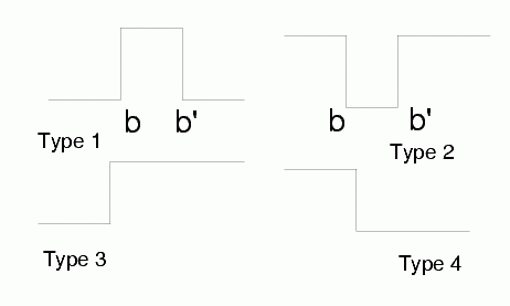
Crisp logic based on rectangular membership functions: True/False values jump from 0 to 1.
Step functions are used for partitioning of the input space.

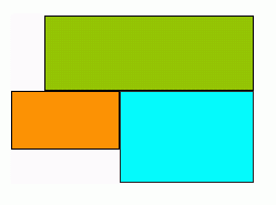
Decision regions: hyperrectangular (cuboidal).

The number of problems that one may analyze using crisp logic may be limited.

Crisp logic rules are most desirable; try them first,
but remember ...

• only one class is predicted P(C_i|X,M) = 0 or 1
  black-and-white picture may be inappropriate in many applications
  
  
• reliable crisp rules may reject some cases as unclassified
  tradeoff: reliability (confidence in rules) - rejection rate
  
  
• discontinuous cost function allow only non-gradient optimization.

Fuzzy logic rules

Property(X)Î [0,1] instead of 0 or 1.
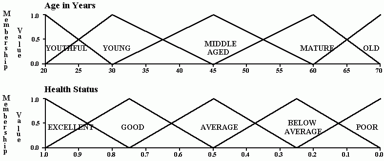
Typical approach: define triangular, trapezoidal, Gaussian and other type of predicate (membership) function.
Membership function m(X) - degree of truth that X has the property m

Frequently features are partitioned by membership functions, defining large receptive fields, reducing information (?).
For example, using triangular functions.

Fuzzy logic: separable functions - products of one-dimensional factors:

Many other possibilities exist to produce N-dimensional membership functions.
Fuzzy rules have continuous membership functions, giving some advantages:

• continuous classification probabilities P(C_i|X,M);
• all vectors classified (some with small probability);
• gradient-based optimization possible;
• sometimes more natural than crisp rules.

But remember ...

• they are not so comprehensible as the crisp rules;
  
  
• danger of overparameterization - more complex rules have additional position/shape parameters.

  

Example: Ljubliana breast cancer

286 cases, 201 no recurrence cancer events (70.3%), 85 are recurrence (29.7%) events.
9 features, symbolic with 2 to 13 values.

Single logical rule:

IF involved nodes >2 AND Degree-malignant=3 THEN recurrence
ELSE norecurrence

gives over 77% accuracy in crossvalidation tests;
best classification systems do not exceed 78% accuracy (insignificant difference).
Some fuzzy/rough systems provided 200 rules with CV accuracy close to the base rate!
Reason: too complex, hard to find simplest solution.

All knowledge contained in the data is:
IF more than 2 areas were infected
AND cancer is highly malignant
THEN there will be recurrence.

• Fixed set of membership functions has less parameters, but fixing the MF shapes is a bad idea!
  Curse of dimensionality:
  k linguistic variables in d dimensions give k^d areas.

  Context-dependent linguistic variables - adapt membership functions in each rule.
  Effect: clusters of different sizes at different input areas.

Problems with rule-based classification models:

• Interpretation of crisp rules may be misleading.
• Predictions using crisp rules are unstable against small perturbations of input values.
• Crisp sets of rules are unstable, small change in the data leads to a large change in the structure of rules.
• Fuzzy rules may be difficult to interpret and do not compress information.
• Fuzzy rules do not estimate real probabilities.
• How to find the best fuzziness/precision tradeoff?

Rules and probabilities

Simplest things first: try crisp rules, large information reduction.

Data from measurements/observations are not precise.
Finite resolution, small receptive fields: Gaussian error distribution:

x => G_x=G(y;x,s_x), where G_x is a Gaussian (fuzzy) number.

Given a set of logical rules {Â} apply them to input data {G_x }.
Use Monte Carlo sampling to recover p(C_i | G_x; {Â }) - may be used with any classifier.

The rule R_a(G_x) = True{x|x>a} is true with probability:

because the cumulant function is approximated by the logistic function:

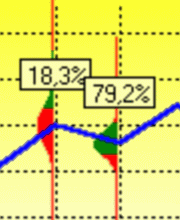
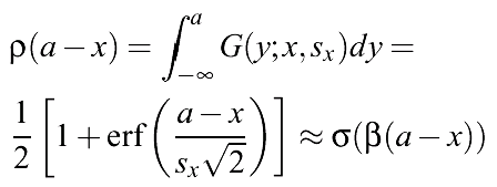
for within 2%

Soft trapezoidal membership functions (MF) realized by neural L-units are obtained.

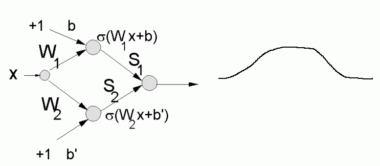
Fuzzy logic with soft trapezoidal MF and crisp inputs is equivalent to crisp logic with G_x inputs;
MLP neural networks with logistic transfer functions provide such MFs.
MLP model includes FL with trapezoidal membership functions.

If rules are overlapping and conditions are correlated the formula leading to Monte Carlo results is:

where 2^Rc are all subsets of the set of classification rules for class C and |R| is the number of rules.
This formula simply avoids counting the same regions twice.

This is not a fuzzy approach!
Here small receptive fields are used, in fuzzy approach a few large receptive fields define linguistic variables.

Benefits:

1. Probabilities instead 0, 1 crisp rule decisions.
2. Vectors that were not classified by crisp rules have now non-zero probabilities.
3. Dispersions S_x may be treated as adaptive parameters of the model M.
4. Gradient methods may be used for large-scale optimization.
   

Next step: optimization of rules exploring the confidence-rejection rate tradeoff.

Define confusion matrix F(C_i,C_j|M) counting the number of cases from class C_j assigned by the set of rules M to the class C_i.

For 2 class problems:

where F_ij is the frequency of cases N_ij / N.
F(C_i,C_j |R) may be defined for a rule or a (sub)set of rules.

Ideal: only the diagonal confusion matrix elements summing to N should be left.

• Minimize sum of the off-diagonals
• Maximize sum of the diagonals
• Combine the two.

Define weighted combination of the number of errors and the "predictive power" of rules:

This should be minimized without constraints; it is bound by -N (number of all training vectors).

Sets of rules M are parameterized by X_k, X'_k intervals.
For g=0 predictive power of rules is maximized.
Rules that make fewer errors on the training data should be more reliable.
Cost function E(M; g) allows to reduce the number of errors to zero (large g) for rules M that reject some instances.

Visualization-based explanation

How to understand the data?

• Create good features: select, combine, use PCA, ICA etc.
• Select linguistic variables as subsets or intervals.
• Extract crisp logical rules.
• Assume small input uncertainty.
• Optimize linguistic variables (and input uncertainty) using the extracted rules.
• Repeat until a stable set of rules is found.

Explanatory data analysis - show the data.
Kohonen's topographics SOM - most popular, trying to classify/display at the same time, but poor in both respects.

Assesing the new data:

• What if our data are not precise?
• How reliable is our classification?
• What other classes are probable?
• Which features are critical?

Investigate the dependence of p(C|G_X; M,S) on S.
If new classes with significant probability appear analyse dependence of p(C|G_X; M,S) on S on individual features X_i.

Example:
with S_i =0 "organic problems'' with 100% confidence;
with 1% uncertainty (optimal, lowest error) "organic problems'' with 90% confidence.
Probabilities of different classes are shown as a function of assumed uncertainties.
S_i=r [Max_i- Min_i], horizontal axis shows r in percents of the input feature range, vertical axis shows probability in percents.

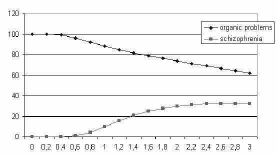
In ambiguous cases probabilities of several new classes quickly rise for growing r and of the most probable class quickly decrease.

PCI, Probabilistic Confidence Intervals

If probability of new classes quickly grows with the assumed uncertainty of the measurement analyze probabilistic confidence levels.
Assume that the value of a single feature is changed, all other are constant; display the two largest probabilities.

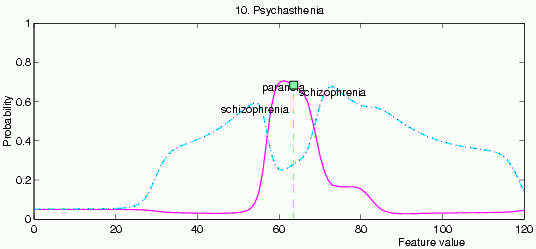
A mixed class appears: paranoidal schizophrenia.

Sensitivity analysis: which feature has strongest influence on the decision?
Shows probabilities in the neighborhood of the case analyzed for a single feature.
Allows to evaluate reliability of classification, but not to explain the data.
May be used with any classifier.
May illustrate the trajectory of changes:

IMDS, Interactive MultiDimensional Scaling

Shows interactively the neighborhood of the case analyzed trying to preserve all topographic relations.
Minimization of a Stress function as:

where w_ij are weights allowing to control which distances are to be better preserved.

Example: focusing on a data point 'p554' from class 'organika'
- Purpose: view (understand) why this data is classified into class 'organika'.
Classified using IncNet neural network, for which features 2, 4 and 7 are sufficient to classify correctly class 'organika'.
Progressive zooming by mapping successively the 200, 100, 50 and 20 nearest data points (interactively selected) from point 'p554' (marked by a black circled dot).

200 nearest neighbors	50 nearest neighbors

Examples of real-life applications

An example of a system based on rules derived from data.

Analysis of psychometric questionnaires

An example of data where logical rules do not work.

Indian Telugu vowel sounds

871 patterns, 6 overlapping vowels, 3 features (formant frequencies).
No reason why simple rules should exist in this case.

Method	Test	Reference
10xCV tests below
3-NN, Manhattan	88.1 ±0.4	Kosice
FSM, 65 Gaussian nodes	87.4 ±0.5	Kosice
SSV dec. tree, 22 rules	86.0	Kosice
2xCV tests below
3-NN, Euclidean	86.1 ±0.6	Kosice
FSM, 40 Gaussian nodes	85.2 ±1.2	Kosice
MLP	84.6	Pal
Fuzzy MLP	84.2	Pal
SSV dec. tree, beam search	83.3 ± 0.9	Kosice
Bayes Classifier	79.2	Pal
Fuzzy SOM	73.5	Pal

More than 20 rules give lower accuracy than kNN.
Simplest explanation: 6 FSM prototypes (one per class), Gaussian weighting of the Euclidean distance.
10xCV gives 72.4% accuracy - insufficient info in the 3 formants.

Conclusions

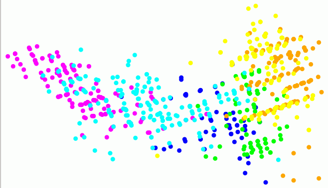
Understanding the data is possible through:

• logical summaries,
• visual displays,
• prototypes.

Rules: frequently rule sets are unstable and/or rule-based classification is unstable.
Small number of accurate rules - best explanation?

Interpretation/evaluation of new cases:

• correlation of rules,
• class probabilities,
• neighborhoods,
• confidence intervals,
• interactive visualization.

Class probabilities may always be estimated by Monte Carlo.
For crisp and most fuzzy rule sets analytical formulas exist.

References

Most papers are available from these pages
http://www.fizyka.umk.pl/kmk/publications.html
http://www.is.umk.pl/~duch/cv/papall.html

Włodzisław Duch